Renewables Case Study: Double Loop Optimization
[1]:
import pyomo.environ as pyo
import idaes

from dispatches_data.api import path
from dispatches.case_studies.renewables_case.wind_battery_double_loop import MultiPeriodWindBattery
from dispatches.case_studies.renewables_case.double_loop_utils import *

for solver in ('xpress_direct', 'gurobi', 'cbc'):
    if pyo.SolverFactory(solver).available(exception_flag=False):
        milp_solver = solver
        break
Creating the Co-simulation of the Wind and Battery IES within the Production Cost Model with Bidder and Tracker Models
In the Conceptual Design Optimization Example Notebook, the design of a Wind + Battery + Hydrogen integrated energy system was optimized using the RTS-GMLC outputs with a “price taker” assumption. Here, we take one of the possible results, a Wind + Battery IES with no Hydrogen, and evaluate its performance in an electricity market by co-simulating its bidding and operation decisions within the production cost model, Prescient, in a “double-loop” optimization.
This double-loop is performed by embedding the multiperiod Wind + Battery flowsheet model as a MultiPeriodWindBattery within a Bidder and a Tracker model, whose functions are to optimize the Day-ahead or Real-time energy market bids, and to optimize the operation of the IES to follow the cleared market’s dispatch, respectively. These functions are coordinated in order and with the correct data transfers with Prescient by a DoubleLoopCoordinator class. Prescient is then able to
evaluate the economic performance of the designed IES within the grid with market interactions and forecast uncertainty. The steps are as shown in this diagram:

In the Day-ahead loop, the Unit Commitment Problem is solved by forecasting loads and obtaining generator bids, and produces hourly schedules and LMPs. The Bidder will use forecasts and plant information to optimize the DA bid to Prescient.
In the Real-time loop, the Economic Dispatch Problem is solved using real-time loads and resources to produce updated generator dispatch points and commitments. The Bidder will use forecasts, DA dispatch and prices, and plant information to optimize the updated RT bid. Once the Real-time market is cleared, the Tracker controls the IES to implement the dispatch at lowest cost.
The market participants are paid on energy and/or reserve provided based on the two-settlement system:
where \(R\) is revenue, \(Q_{DA}\) is power sold to DA market at \(P_{DA}\) price, and \(Q_{RT}\) is power delivered to RT market at \(P_{RT}\) price.
First, we define the electricity grid for the double-loop simulation via options to Prescient: the directory to the RTS-GMLC source data, the time horizons for the UC and ED problems, the start date and length of the simulation, how much reserves should be procured, etc. The full-year PCM simulation was completed prior and the outputs were collected into a 309_WIND_1-SimulationOutputs.csv in order to provide “historical” LMPs and Wind resource capacity factors for the Conceptual Design
Optimization.
In this example, we will repeat the Prescient simulation with no reserves for a single week, where the Wind + Battery IES will replace the 309_WIND_1 Wind plant at the “Carter” bus.
[2]:
from prescient.simulator import Prescient
import os

TESTING_MODE = bool(os.environ.get("DISPATCHES_TESTING_MODE", None))
rts_gmlc_source_data_path = path("rts_gmlc") / "SourceData"

sim_days = 7 if not TESTING_MODE else 1
start_date = "01-02-2020"
day_ahead_horizon = 28
real_time_horizon = 4
output_dir = Path(f"double_loop_results")

wind_bus = 309
wind_bus_name = "Carter"
wind_generator = f"{wind_bus}_WIND_1"

prescient_options = {
    "data_path": str(rts_gmlc_source_data_path),
    "input_format": "rts-gmlc",
    "simulate_out_of_sample": True,
    "run_sced_with_persistent_forecast_errors": True,
    "output_directory": output_dir,
    "start_date": start_date,
    "num_days": sim_days,
    "sced_horizon": real_time_horizon,
    "ruc_horizon": day_ahead_horizon,
    "ruc_every_hours": 24,
    "compute_market_settlements": True,
    "day_ahead_pricing": "LMP",
    "ruc_mipgap": 0.05 if not TESTING_MODE else 0.5,
    "symbolic_solver_labels": True,
    "reserve_factor": 0,
    "deterministic_ruc_solver": milp_solver,
    "sced_solver": milp_solver,
    "plugin": {
        "doubleloop": {
            "module": None,                                          # to be added below
            "bidding_generator": wind_generator,
        }
    }
}

# collect "historical" full-year wind forecast and first-day LMPs
prescient_outputs_df = pd.read_csv(Path(os.path.realpath("__file__")).parent / "data" / "309_WIND_1-SimulationOutputs.csv")
prescient_outputs_df.index = pd.to_datetime(prescient_outputs_df['Unnamed: 0'])
prescient_outputs_df = prescient_outputs_df[prescient_outputs_df.index >= pd.Timestamp(f'{start_date} 00:00:00')]
gen_capacity_factor = prescient_outputs_df[f"{wind_generator}-RTCF"].values.tolist()
historical_da_prices = {
    wind_bus_name: prescient_outputs_df[f"LMP DA"].values[0:24].tolist()
}
historical_rt_prices = {
    wind_bus_name: prescient_outputs_df[f"LMP"].values[0:24].tolist()
}
Interactive Python mode detected; using default matplotlib backend for plotting.
[3]:
from matplotlib.ticker import MultipleLocator
import matplotlib.pyplot as plt
plt.rcParams.update({'font.size': 16, 'axes.titlesize': 16, 'axes.labelsize': 14})

def format_plt(fig, ax, titles, suptitle=None, mod_ticks=True, y_labels=None):
    if not y_labels:
        y_labels = ["Power [MW]"] * len(ax)
    for i in range(len(ax)):
        if mod_ticks:
            ax[i].xaxis.set_minor_locator(MultipleLocator(4))
            ax[i].xaxis.set_major_locator(MultipleLocator(24))
            ax[i].tick_params(axis='both', which='major', labelsize="small")
            ax[i].tick_params(axis='both', which='minor', labelsize="small")
        ax[i].legend()
        ax[i].set_ylabel(y_labels[i])
        ax[i].set_xlabel("Time [hr]")
        ax[i].set_title(titles[i])
    fig.autofmt_xdate(rotation=45)
    if suptitle:
        fig.suptitle(suptitle)
    fig.tight_layout()

time_index = prescient_outputs_df[prescient_outputs_df.index <= prescient_outputs_df.index[24 * sim_days]].index
orig_outputs_df = prescient_outputs_df[prescient_outputs_df.index.isin(time_index)].copy()
orig_outputs_df['Penalized DA Underdelivered [MW]'] = (orig_outputs_df['Output DA'] - orig_outputs_df['Output']) * (orig_outputs_df['LMP'] > orig_outputs_df['LMP DA'])
orig_outputs_df.loc[:, 'Penalized DA Underdelivered [MW]'].clip(lower=0, inplace=True)
orig_outputs_df['Curtailment'] *= -1

fig, ax = plt.subplots(2, 1, figsize=(24, 10), sharex=True)
ax[0].plot(orig_outputs_df['Output DA'].values, drawstyle="steps-mid", label='DA Dispatch [MW]', color='grey')
ax[0].plot(orig_outputs_df['Output'].values, drawstyle="steps-mid", label='RT Dispatch [MW]', color='k')
cols = ['Output', 'Penalized DA Underdelivered [MW]']
orig_outputs_df[cols].plot(kind='bar', width=1, stacked=True, ax=ax[0], color=['b', 'r'])
orig_outputs_df['Curtailment'].plot(kind='bar', width=1, stacked=True, ax=ax[1])
format_plt(fig, ax, titles=["Wind Output vs Dispatch", "Wind Curtailment"], suptitle="Original RTS-GMLC Simulation")
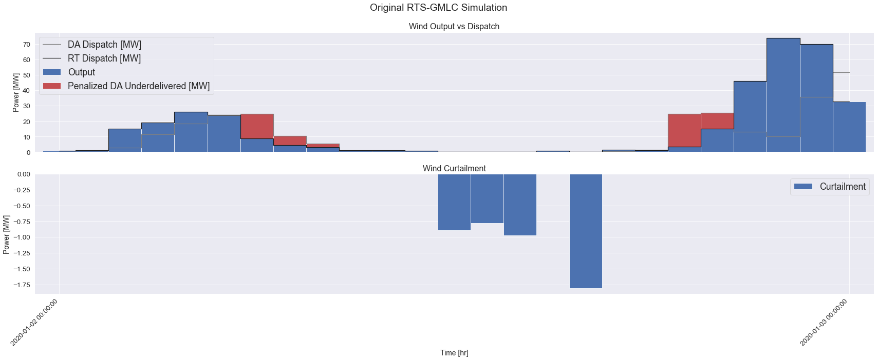
The above plot shows the wind plant’s DA Dispatch, RT Dispatch, Wind Power Output, Penalized DA Underdelivered, and Wind Curtailment in MW for the first week. The DA and RT Dispatch profiles are from the final solution of Prescient’s staggered and forward-rolling UC and ED problems, and are based on the day-ahead and real-time wind forecast, respectively.
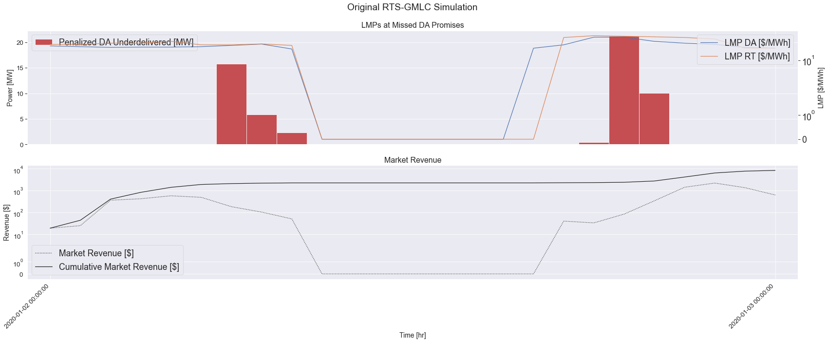
The Wind Power Output is the real-time wind production of the wind plant, and matches the RT Dispatch exactly. However, since there was uncertainty of the RT wind resource during the DA bid, the DA Dispatch is different. According to the two-settlement system revenue equation above, the wind plant will be charged the RT LMP for the difference between the promised DA Dispatch and the delivered RT power. The Penalized DA Underdelivered profile show the power that was underdelivered
when RT LMPs were higher than DA LMPs and resulted in some negative revenue for the plant.
The second plot below shows the Hourly and Cumulative revenue of the wind plant.
[4]:
fig, ax = plt.subplots(2, 1, figsize=(24, 10), sharex=True)

orig_outputs_df['Penalized DA Underdelivered [MW]'].plot(ax=ax[0], color='r', kind='bar', width=1)
ax0 = ax[0].twinx()
ax0.set_yscale('symlog')
ax0.plot(orig_outputs_df['LMP DA'].values, label="LMP DA [$/MWh]")
ax0.plot(orig_outputs_df['LMP'].values, label='LMP RT [$/MWh]')
ax0.legend(loc='upper right')
ax0.grid(None)
ax0.set_ylabel("LMP [$/MWh]")
ax[1].set_yscale('symlog')
ax[1].plot(orig_outputs_df['Unit Market Revenue'].values, color='k', linestyle=':', label="Market Revenue [$]")
ax[1].plot(orig_outputs_df['Unit Market Revenue'].cumsum().values, color='k', label="Cumulative Market Revenue [$]")

format_plt(fig, ax, y_labels=['Power [MW]', 'Revenue [$]'], titles=["LMPs at Missed DA Promises", "Market Revenue"], suptitle="Original RTS-GMLC Simulation")
ax[0].legend(loc='upper left')
[4]:
<matplotlib.legend.Legend at 0x7fd48ade8cd0>
Creating the IES Generator within the RTS-GMLC
First, the location, type, capacity, and other parameters of the IES needs to be defined in order to situate the generator within the electricity market. In this example, the IES’ bid will be represented as that of a thermal generator, with parameters such as min power, max power, ramping constraints, startup and shutdown capacity, even though the IES will not need them all. The wind resource at the chosen location, at the “Carter” bus, is read from the RTS-GMLC Source Data.
The information is passed to the MultiPeriodWindBattery class, which enables the Bidder and Tracker to construct a Wind + Battery multiperiod model within its bidding and tracking optimization problems via populate_model, and to update the state of the Wind + Battery IES as the double-loop steps forward in time via update_model.
[5]:
from idaes.apps.grid_integration.model_data import ThermalGeneratorModelData

p_min = 0
wind_pmax = 147.6
battery_pmax = 25
battery_emax = battery_pmax * 4

# for descriptions on what each parameter means, see `help(ThermalGeneratorModelData)`
thermal_generator_params = {
    "gen_name": wind_generator,
    "bus": wind_bus_name,
    "p_min": p_min,
    "p_max": wind_pmax,
    "min_down_time": 0,
    "min_up_time": 0,
    "ramp_up_60min": wind_pmax + battery_pmax,
    "ramp_down_60min": wind_pmax + battery_pmax,
    "shutdown_capacity": wind_pmax + battery_pmax,
    "startup_capacity": 0,
    "initial_status": 1,
    "initial_p_output": 0,
    "production_cost_bid_pairs": [(p_min, 0), (wind_pmax, 0)],
    "include_default_p_cost": False,
    "startup_cost_pairs": [(0, 0)],
    "fixed_commitment": 1,
}
model_data = ThermalGeneratorModelData(**thermal_generator_params)

mp_wind_battery_bid = MultiPeriodWindBattery(
    model_data=model_data,
    wind_capacity_factors=gen_capacity_factor,
    wind_pmax_mw=wind_pmax,
    battery_pmax_mw=battery_pmax,
    battery_energy_capacity_mwh=battery_emax,
)
Creating the Forecaster, Tracker, and Bidder for the DoupleLoopCoordinator
The Bidder requires a forecast of the DA and RT prices in order to plan out its energy bid: at what time to sell how much energy and at what price, given the anticipated wind resource and the evolution of the battery state-of-charge. In contrast to the price-taker assumption in the Conceptual Design phase where the Wind + Battery IES took the historical LMPs for however much energy it sold, here, the Bidder does not know what the final LMP will be, nor that its bid for energy at a
certain marginal cost will be accepted by the market.
The Backcaster class stores historical DA and RT LMPs in order to generate forecast scenarios. The first day of simulated DA and RT LMPs initializes the Backcaster, which continues to collect resolved LMPs as the simulation steps forward in time.
Within the DoubleLoopCoordinator, there are two Tracker objects, the first tracker follows the real-time market signals whereas the second projection_tracker projects the latest real-time dispatch onto the next day-ahead bidding problem.
[6]:
from idaes.apps.grid_integration.forecaster import Backcaster
from idaes.apps.grid_integration import Tracker, Bidder
from dispatches.workflow.coordinator import DoubleLoopCoordinator

# Backcaster
# help(Backcaster)
backcaster = Backcaster(historical_da_prices, historical_rt_prices)
[7]:
n_price_scenario = 3
solver = pyo.SolverFactory(milp_solver)

# Bidder
# help(Bidder)
bidder_mp_wind_battery = MultiPeriodWindBattery(
    model_data=model_data,
    wind_capacity_factors=gen_capacity_factor,
    wind_pmax_mw=wind_pmax,
    battery_pmax_mw=battery_pmax,
    battery_energy_capacity_mwh=battery_emax,
)

bidder_object = Bidder(
    bidding_model_object=bidder_mp_wind_battery,
    day_ahead_horizon=day_ahead_horizon,
    real_time_horizon=real_time_horizon,
    n_scenario=n_price_scenario,
    solver=solver,
    forecaster=backcaster,
)
[+   0.00] Beginning the formulation of the multiperiod optimization problem.
2023-03-14 15:23:01 [INFO] idaes.apps.grid_integration.multiperiod.multiperiod: ...Constructing the flowsheet model for blocks[0]
WARNING: model contains export suffix 'fs.splitter.scaling_factor' that
    contains 4 component keys that are not exported as part of the NL file.
    Skipping.
2023-03-14 15:23:02 [INFO] idaes.apps.grid_integration.multiperiod.multiperiod: ...Constructing the flowsheet model for blocks[1]
2023-03-14 15:23:02 [INFO] idaes.apps.grid_integration.multiperiod.multiperiod: ...Constructing the flowsheet model for blocks[2]
2023-03-14 15:23:02 [INFO] idaes.apps.grid_integration.multiperiod.multiperiod: ...Constructing the flowsheet model for blocks[3]
2023-03-14 15:23:02 [INFO] idaes.apps.grid_integration.multiperiod.multiperiod: ...Constructing the flowsheet model for blocks[4]
2023-03-14 15:23:02 [INFO] idaes.apps.grid_integration.multiperiod.multiperiod: ...Constructing the flowsheet model for blocks[5]
2023-03-14 15:23:02 [INFO] idaes.apps.grid_integration.multiperiod.multiperiod: ...Constructing the flowsheet model for blocks[6]
2023-03-14 15:23:02 [INFO] idaes.apps.grid_integration.multiperiod.multiperiod: ...Constructing the flowsheet model for blocks[7]
2023-03-14 15:23:02 [INFO] idaes.apps.grid_integration.multiperiod.multiperiod: ...Constructing the flowsheet model for blocks[8]
2023-03-14 15:23:02 [INFO] idaes.apps.grid_integration.multiperiod.multiperiod: ...Constructing the flowsheet model for blocks[9]
2023-03-14 15:23:02 [INFO] idaes.apps.grid_integration.multiperiod.multiperiod: ...Constructing the flowsheet model for blocks[10]
2023-03-14 15:23:02 [INFO] idaes.apps.grid_integration.multiperiod.multiperiod: ...Constructing the flowsheet model for blocks[11]
2023-03-14 15:23:02 [INFO] idaes.apps.grid_integration.multiperiod.multiperiod: ...Constructing the flowsheet model for blocks[12]
2023-03-14 15:23:02 [INFO] idaes.apps.grid_integration.multiperiod.multiperiod: ...Constructing the flowsheet model for blocks[13]
2023-03-14 15:23:02 [INFO] idaes.apps.grid_integration.multiperiod.multiperiod: ...Constructing the flowsheet model for blocks[14]
2023-03-14 15:23:02 [INFO] idaes.apps.grid_integration.multiperiod.multiperiod: ...Constructing the flowsheet model for blocks[15]
2023-03-14 15:23:02 [INFO] idaes.apps.grid_integration.multiperiod.multiperiod: ...Constructing the flowsheet model for blocks[16]
2023-03-14 15:23:02 [INFO] idaes.apps.grid_integration.multiperiod.multiperiod: ...Constructing the flowsheet model for blocks[17]
2023-03-14 15:23:02 [INFO] idaes.apps.grid_integration.multiperiod.multiperiod: ...Constructing the flowsheet model for blocks[18]
2023-03-14 15:23:02 [INFO] idaes.apps.grid_integration.multiperiod.multiperiod: ...Constructing the flowsheet model for blocks[19]
2023-03-14 15:23:02 [INFO] idaes.apps.grid_integration.multiperiod.multiperiod: ...Constructing the flowsheet model for blocks[20]
2023-03-14 15:23:02 [INFO] idaes.apps.grid_integration.multiperiod.multiperiod: ...Constructing the flowsheet model for blocks[21]
2023-03-14 15:23:02 [INFO] idaes.apps.grid_integration.multiperiod.multiperiod: ...Constructing the flowsheet model for blocks[22]
2023-03-14 15:23:02 [INFO] idaes.apps.grid_integration.multiperiod.multiperiod: ...Constructing the flowsheet model for blocks[23]
2023-03-14 15:23:02 [INFO] idaes.apps.grid_integration.multiperiod.multiperiod: ...Constructing the flowsheet model for blocks[24]
2023-03-14 15:23:02 [INFO] idaes.apps.grid_integration.multiperiod.multiperiod: ...Constructing the flowsheet model for blocks[25]
2023-03-14 15:23:02 [INFO] idaes.apps.grid_integration.multiperiod.multiperiod: ...Constructing the flowsheet model for blocks[26]
2023-03-14 15:23:02 [INFO] idaes.apps.grid_integration.multiperiod.multiperiod: ...Constructing the flowsheet model for blocks[27]
[+   0.66] Completed the formulation of the multiperiod optimization problem.
2023-03-14 15:23:02 [WARNING] idaes.apps.grid_integration.multiperiod.multiperiod: Initialization function is not provided. Returning the multiperiod model without initialization.
2023-03-14 15:23:02 [WARNING] idaes.apps.grid_integration.multiperiod.multiperiod: unfix_dof function is not provided. Returning the model without unfixing degrees of freedom
[+   0.00] Beginning the formulation of the multiperiod optimization problem.
2023-03-14 15:23:02 [INFO] idaes.apps.grid_integration.multiperiod.multiperiod: ...Constructing the flowsheet model for blocks[0]
WARNING: model contains export suffix 'fs.splitter.scaling_factor' that
    contains 4 component keys that are not exported as part of the NL file.
    Skipping.
2023-03-14 15:23:02 [INFO] idaes.apps.grid_integration.multiperiod.multiperiod: ...Constructing the flowsheet model for blocks[1]
2023-03-14 15:23:02 [INFO] idaes.apps.grid_integration.multiperiod.multiperiod: ...Constructing the flowsheet model for blocks[2]
2023-03-14 15:23:02 [INFO] idaes.apps.grid_integration.multiperiod.multiperiod: ...Constructing the flowsheet model for blocks[3]
2023-03-14 15:23:02 [INFO] idaes.apps.grid_integration.multiperiod.multiperiod: ...Constructing the flowsheet model for blocks[4]
2023-03-14 15:23:02 [INFO] idaes.apps.grid_integration.multiperiod.multiperiod: ...Constructing the flowsheet model for blocks[5]
2023-03-14 15:23:02 [INFO] idaes.apps.grid_integration.multiperiod.multiperiod: ...Constructing the flowsheet model for blocks[6]
2023-03-14 15:23:02 [INFO] idaes.apps.grid_integration.multiperiod.multiperiod: ...Constructing the flowsheet model for blocks[7]
2023-03-14 15:23:02 [INFO] idaes.apps.grid_integration.multiperiod.multiperiod: ...Constructing the flowsheet model for blocks[8]
2023-03-14 15:23:02 [INFO] idaes.apps.grid_integration.multiperiod.multiperiod: ...Constructing the flowsheet model for blocks[9]
2023-03-14 15:23:02 [INFO] idaes.apps.grid_integration.multiperiod.multiperiod: ...Constructing the flowsheet model for blocks[10]
2023-03-14 15:23:02 [INFO] idaes.apps.grid_integration.multiperiod.multiperiod: ...Constructing the flowsheet model for blocks[11]
2023-03-14 15:23:02 [INFO] idaes.apps.grid_integration.multiperiod.multiperiod: ...Constructing the flowsheet model for blocks[12]
2023-03-14 15:23:02 [INFO] idaes.apps.grid_integration.multiperiod.multiperiod: ...Constructing the flowsheet model for blocks[13]
2023-03-14 15:23:02 [INFO] idaes.apps.grid_integration.multiperiod.multiperiod: ...Constructing the flowsheet model for blocks[14]
2023-03-14 15:23:02 [INFO] idaes.apps.grid_integration.multiperiod.multiperiod: ...Constructing the flowsheet model for blocks[15]
2023-03-14 15:23:02 [INFO] idaes.apps.grid_integration.multiperiod.multiperiod: ...Constructing the flowsheet model for blocks[16]
2023-03-14 15:23:02 [INFO] idaes.apps.grid_integration.multiperiod.multiperiod: ...Constructing the flowsheet model for blocks[17]
2023-03-14 15:23:03 [INFO] idaes.apps.grid_integration.multiperiod.multiperiod: ...Constructing the flowsheet model for blocks[18]
2023-03-14 15:23:03 [INFO] idaes.apps.grid_integration.multiperiod.multiperiod: ...Constructing the flowsheet model for blocks[19]
2023-03-14 15:23:03 [INFO] idaes.apps.grid_integration.multiperiod.multiperiod: ...Constructing the flowsheet model for blocks[20]
2023-03-14 15:23:03 [INFO] idaes.apps.grid_integration.multiperiod.multiperiod: ...Constructing the flowsheet model for blocks[21]
2023-03-14 15:23:03 [INFO] idaes.apps.grid_integration.multiperiod.multiperiod: ...Constructing the flowsheet model for blocks[22]
2023-03-14 15:23:03 [INFO] idaes.apps.grid_integration.multiperiod.multiperiod: ...Constructing the flowsheet model for blocks[23]
2023-03-14 15:23:03 [INFO] idaes.apps.grid_integration.multiperiod.multiperiod: ...Constructing the flowsheet model for blocks[24]
2023-03-14 15:23:03 [INFO] idaes.apps.grid_integration.multiperiod.multiperiod: ...Constructing the flowsheet model for blocks[25]
2023-03-14 15:23:03 [INFO] idaes.apps.grid_integration.multiperiod.multiperiod: ...Constructing the flowsheet model for blocks[26]
2023-03-14 15:23:03 [INFO] idaes.apps.grid_integration.multiperiod.multiperiod: ...Constructing the flowsheet model for blocks[27]
[+   0.55] Completed the formulation of the multiperiod optimization problem.
2023-03-14 15:23:03 [WARNING] idaes.apps.grid_integration.multiperiod.multiperiod: Initialization function is not provided. Returning the multiperiod model without initialization.
2023-03-14 15:23:03 [WARNING] idaes.apps.grid_integration.multiperiod.multiperiod: unfix_dof function is not provided. Returning the model without unfixing degrees of freedom
[+   0.00] Beginning the formulation of the multiperiod optimization problem.
2023-03-14 15:23:03 [INFO] idaes.apps.grid_integration.multiperiod.multiperiod: ...Constructing the flowsheet model for blocks[0]
WARNING: model contains export suffix 'fs.splitter.scaling_factor' that
    contains 4 component keys that are not exported as part of the NL file.
    Skipping.
2023-03-14 15:23:03 [INFO] idaes.apps.grid_integration.multiperiod.multiperiod: ...Constructing the flowsheet model for blocks[1]
2023-03-14 15:23:03 [INFO] idaes.apps.grid_integration.multiperiod.multiperiod: ...Constructing the flowsheet model for blocks[2]
2023-03-14 15:23:03 [INFO] idaes.apps.grid_integration.multiperiod.multiperiod: ...Constructing the flowsheet model for blocks[3]
2023-03-14 15:23:03 [INFO] idaes.apps.grid_integration.multiperiod.multiperiod: ...Constructing the flowsheet model for blocks[4]
2023-03-14 15:23:03 [INFO] idaes.apps.grid_integration.multiperiod.multiperiod: ...Constructing the flowsheet model for blocks[5]
2023-03-14 15:23:03 [INFO] idaes.apps.grid_integration.multiperiod.multiperiod: ...Constructing the flowsheet model for blocks[6]
2023-03-14 15:23:03 [INFO] idaes.apps.grid_integration.multiperiod.multiperiod: ...Constructing the flowsheet model for blocks[7]
2023-03-14 15:23:03 [INFO] idaes.apps.grid_integration.multiperiod.multiperiod: ...Constructing the flowsheet model for blocks[8]
2023-03-14 15:23:03 [INFO] idaes.apps.grid_integration.multiperiod.multiperiod: ...Constructing the flowsheet model for blocks[9]
2023-03-14 15:23:03 [INFO] idaes.apps.grid_integration.multiperiod.multiperiod: ...Constructing the flowsheet model for blocks[10]
2023-03-14 15:23:03 [INFO] idaes.apps.grid_integration.multiperiod.multiperiod: ...Constructing the flowsheet model for blocks[11]
2023-03-14 15:23:03 [INFO] idaes.apps.grid_integration.multiperiod.multiperiod: ...Constructing the flowsheet model for blocks[12]
2023-03-14 15:23:03 [INFO] idaes.apps.grid_integration.multiperiod.multiperiod: ...Constructing the flowsheet model for blocks[13]
2023-03-14 15:23:03 [INFO] idaes.apps.grid_integration.multiperiod.multiperiod: ...Constructing the flowsheet model for blocks[14]
2023-03-14 15:23:03 [INFO] idaes.apps.grid_integration.multiperiod.multiperiod: ...Constructing the flowsheet model for blocks[15]
2023-03-14 15:23:03 [INFO] idaes.apps.grid_integration.multiperiod.multiperiod: ...Constructing the flowsheet model for blocks[16]
2023-03-14 15:23:03 [INFO] idaes.apps.grid_integration.multiperiod.multiperiod: ...Constructing the flowsheet model for blocks[17]
2023-03-14 15:23:03 [INFO] idaes.apps.grid_integration.multiperiod.multiperiod: ...Constructing the flowsheet model for blocks[18]
2023-03-14 15:23:03 [INFO] idaes.apps.grid_integration.multiperiod.multiperiod: ...Constructing the flowsheet model for blocks[19]
2023-03-14 15:23:03 [INFO] idaes.apps.grid_integration.multiperiod.multiperiod: ...Constructing the flowsheet model for blocks[20]
2023-03-14 15:23:03 [INFO] idaes.apps.grid_integration.multiperiod.multiperiod: ...Constructing the flowsheet model for blocks[21]
2023-03-14 15:23:03 [INFO] idaes.apps.grid_integration.multiperiod.multiperiod: ...Constructing the flowsheet model for blocks[22]
2023-03-14 15:23:03 [INFO] idaes.apps.grid_integration.multiperiod.multiperiod: ...Constructing the flowsheet model for blocks[23]
2023-03-14 15:23:03 [INFO] idaes.apps.grid_integration.multiperiod.multiperiod: ...Constructing the flowsheet model for blocks[24]
2023-03-14 15:23:03 [INFO] idaes.apps.grid_integration.multiperiod.multiperiod: ...Constructing the flowsheet model for blocks[25]
2023-03-14 15:23:03 [INFO] idaes.apps.grid_integration.multiperiod.multiperiod: ...Constructing the flowsheet model for blocks[26]
2023-03-14 15:23:03 [INFO] idaes.apps.grid_integration.multiperiod.multiperiod: ...Constructing the flowsheet model for blocks[27]
[+   0.55] Completed the formulation of the multiperiod optimization problem.
2023-03-14 15:23:03 [WARNING] idaes.apps.grid_integration.multiperiod.multiperiod: Initialization function is not provided. Returning the multiperiod model without initialization.
2023-03-14 15:23:03 [WARNING] idaes.apps.grid_integration.multiperiod.multiperiod: unfix_dof function is not provided. Returning the model without unfixing degrees of freedom
[+   0.00] Beginning the formulation of the multiperiod optimization problem.
2023-03-14 15:23:03 [INFO] idaes.apps.grid_integration.multiperiod.multiperiod: ...Constructing the flowsheet model for blocks[0]
WARNING: model contains export suffix 'fs.splitter.scaling_factor' that
    contains 4 component keys that are not exported as part of the NL file.
    Skipping.
2023-03-14 15:23:03 [INFO] idaes.apps.grid_integration.multiperiod.multiperiod: ...Constructing the flowsheet model for blocks[1]
2023-03-14 15:23:03 [INFO] idaes.apps.grid_integration.multiperiod.multiperiod: ...Constructing the flowsheet model for blocks[2]
2023-03-14 15:23:04 [INFO] idaes.apps.grid_integration.multiperiod.multiperiod: ...Constructing the flowsheet model for blocks[3]
[+   0.28] Completed the formulation of the multiperiod optimization problem.
2023-03-14 15:23:04 [WARNING] idaes.apps.grid_integration.multiperiod.multiperiod: Initialization function is not provided. Returning the multiperiod model without initialization.
2023-03-14 15:23:04 [WARNING] idaes.apps.grid_integration.multiperiod.multiperiod: unfix_dof function is not provided. Returning the model without unfixing degrees of freedom
[+   0.00] Beginning the formulation of the multiperiod optimization problem.
2023-03-14 15:23:04 [INFO] idaes.apps.grid_integration.multiperiod.multiperiod: ...Constructing the flowsheet model for blocks[0]
WARNING: model contains export suffix 'fs.splitter.scaling_factor' that
    contains 4 component keys that are not exported as part of the NL file.
    Skipping.
2023-03-14 15:23:04 [INFO] idaes.apps.grid_integration.multiperiod.multiperiod: ...Constructing the flowsheet model for blocks[1]
2023-03-14 15:23:04 [INFO] idaes.apps.grid_integration.multiperiod.multiperiod: ...Constructing the flowsheet model for blocks[2]
2023-03-14 15:23:04 [INFO] idaes.apps.grid_integration.multiperiod.multiperiod: ...Constructing the flowsheet model for blocks[3]
[+   0.12] Completed the formulation of the multiperiod optimization problem.
2023-03-14 15:23:04 [WARNING] idaes.apps.grid_integration.multiperiod.multiperiod: Initialization function is not provided. Returning the multiperiod model without initialization.
2023-03-14 15:23:04 [WARNING] idaes.apps.grid_integration.multiperiod.multiperiod: unfix_dof function is not provided. Returning the model without unfixing degrees of freedom
[+   0.00] Beginning the formulation of the multiperiod optimization problem.
2023-03-14 15:23:04 [INFO] idaes.apps.grid_integration.multiperiod.multiperiod: ...Constructing the flowsheet model for blocks[0]
WARNING: model contains export suffix 'fs.splitter.scaling_factor' that
    contains 4 component keys that are not exported as part of the NL file.
    Skipping.
2023-03-14 15:23:04 [INFO] idaes.apps.grid_integration.multiperiod.multiperiod: ...Constructing the flowsheet model for blocks[1]
2023-03-14 15:23:04 [INFO] idaes.apps.grid_integration.multiperiod.multiperiod: ...Constructing the flowsheet model for blocks[2]
2023-03-14 15:23:04 [INFO] idaes.apps.grid_integration.multiperiod.multiperiod: ...Constructing the flowsheet model for blocks[3]
[+   0.18] Completed the formulation of the multiperiod optimization problem.
2023-03-14 15:23:04 [WARNING] idaes.apps.grid_integration.multiperiod.multiperiod: Initialization function is not provided. Returning the multiperiod model without initialization.
2023-03-14 15:23:04 [WARNING] idaes.apps.grid_integration.multiperiod.multiperiod: unfix_dof function is not provided. Returning the model without unfixing degrees of freedom
[8]:
tracking_horizon = 4
n_tracking_hour = 1

# Tracker
# help(Tracker)
tracker_mp_wind_battery = MultiPeriodWindBattery(
    model_data=model_data,
    wind_capacity_factors=gen_capacity_factor,
    wind_pmax_mw=wind_pmax,
    battery_pmax_mw=battery_pmax,
    battery_energy_capacity_mwh=battery_emax,
)

tracker_object = Tracker(
    tracking_model_object=tracker_mp_wind_battery,
    tracking_horizon=tracking_horizon,
    n_tracking_hour=n_tracking_hour,
    solver=solver,
)

# Projection Tracker
projection_mp_wind_battery = MultiPeriodWindBattery(
    model_data=model_data,
    wind_capacity_factors=gen_capacity_factor,
    wind_pmax_mw=wind_pmax,
    battery_pmax_mw=battery_pmax,
    battery_energy_capacity_mwh=battery_emax,
)

projection_tracker_object = Tracker(
    tracking_model_object=projection_mp_wind_battery,
    tracking_horizon=tracking_horizon,
    n_tracking_hour=n_tracking_hour,
    solver=solver,
)
[+   0.00] Beginning the formulation of the multiperiod optimization problem.
2023-03-14 15:23:04 [INFO] idaes.apps.grid_integration.multiperiod.multiperiod: ...Constructing the flowsheet model for blocks[0]
WARNING: model contains export suffix 'fs.splitter.scaling_factor' that
    contains 4 component keys that are not exported as part of the NL file.
    Skipping.
2023-03-14 15:23:04 [INFO] idaes.apps.grid_integration.multiperiod.multiperiod: ...Constructing the flowsheet model for blocks[1]
2023-03-14 15:23:04 [INFO] idaes.apps.grid_integration.multiperiod.multiperiod: ...Constructing the flowsheet model for blocks[2]
2023-03-14 15:23:04 [INFO] idaes.apps.grid_integration.multiperiod.multiperiod: ...Constructing the flowsheet model for blocks[3]
[+   0.18] Completed the formulation of the multiperiod optimization problem.
2023-03-14 15:23:04 [WARNING] idaes.apps.grid_integration.multiperiod.multiperiod: Initialization function is not provided. Returning the multiperiod model without initialization.
2023-03-14 15:23:04 [WARNING] idaes.apps.grid_integration.multiperiod.multiperiod: unfix_dof function is not provided. Returning the model without unfixing degrees of freedom
[+   0.00] Beginning the formulation of the multiperiod optimization problem.
2023-03-14 15:23:04 [INFO] idaes.apps.grid_integration.multiperiod.multiperiod: ...Constructing the flowsheet model for blocks[0]
WARNING: model contains export suffix 'fs.splitter.scaling_factor' that
    contains 4 component keys that are not exported as part of the NL file.
    Skipping.
2023-03-14 15:23:04 [INFO] idaes.apps.grid_integration.multiperiod.multiperiod: ...Constructing the flowsheet model for blocks[1]
2023-03-14 15:23:04 [INFO] idaes.apps.grid_integration.multiperiod.multiperiod: ...Constructing the flowsheet model for blocks[2]
2023-03-14 15:23:04 [INFO] idaes.apps.grid_integration.multiperiod.multiperiod: ...Constructing the flowsheet model for blocks[3]
[+   0.17] Completed the formulation of the multiperiod optimization problem.
2023-03-14 15:23:04 [WARNING] idaes.apps.grid_integration.multiperiod.multiperiod: Initialization function is not provided. Returning the multiperiod model without initialization.
2023-03-14 15:23:04 [WARNING] idaes.apps.grid_integration.multiperiod.multiperiod: unfix_dof function is not provided. Returning the model without unfixing degrees of freedom
[9]:
# Compose into Coordinator
# help(DoubleLoopCoordinator)
coordinator = DoubleLoopCoordinator(
    bidder=bidder_object,
    tracker=tracker_object,
    projection_tracker=projection_tracker_object,
)
Running the Double-Loop Plugin
The prescient_options are updated with the DoubleLoopCoordinator. The simulation results will be written to the output_dir folder.
[10]:
import shutil

prescient_options['plugin']['doubleloop']['module'] = coordinator.prescient_plugin_module

if output_dir.exists():
    shutil.rmtree(output_dir)

Prescient().simulate(**prescient_options)
Initializing simulation...
Did not find reserves.csv; assuming no reserves
/Users/dguittet/miniconda3/envs/dispatches/lib/python3.8/site-packages/pandas/io/parsers/base_parser.py:1055: FutureWarning:
        Use pd.to_datetime instead.

  return generic_parser(date_parser, *date_cols)
Setting default t0 state in RTS-GMLC parser
Dates to simulate: 2020-01-02 to 2020-01-02
RUC activation hours: 0
Final RUC date: 2020-01-02
Using current day's forecasts for RUC solves
Using persistent forecast error model when projecting demand and renewables in SCED
Extracting scenario to simulate
FICO Xpress v8.12.4, Hyper, solve started 15:23:10, Mar 14, 2023
Heap usage: 953KB (peak 1073KB, 1176KB system)
Maximizing LP unknown with these control settings:
OUTPUTLOG = 1
Original problem has:
1506 rows 1260 cols 2583 elements
Presolved problem has:
249 rows 336 cols 831 elements
Presolve finished in 0 seconds
Heap usage: 1050KB (peak 1969KB, 1178KB system)
Coefficient range original solved
Coefficients [min,max] : [ 1.00e-04, 1.05e+00] / [ 1.56e-02, 1.60e+01]
RHS and bounds [min,max] : [ 7.71e+02, 1.00e+08] / [ 7.71e+02, 8.00e+08]
Objective [min,max] : [ 1.50e-02, 1.89e+01] / [ 7.50e-03, 1.20e-01]
Autoscaling applied Curtis-Reid scaling
Crash basis containing 21 structural columns created
Its Obj Value S Ninf Nneg Sum Dual Inf Time
0 16961.67995 D 1 3 .720000 0
182 -19382.55330 D 0 0 .000000 0
Uncrunching matrix
Optimal solution found
Dual solved problem
182 simplex iterations in 0.00 seconds at time 0
Final objective : -1.938255330232465e+04
Max primal violation (abs/rel) : 0.0 / 0.0
Max dual violation (abs/rel) : 0.0 / 0.0
Max complementarity viol. (abs/rel) : 0.0 / 0.0
Calculating PTDF Matrix Factorization
Pyomo model construction time: 3.34
User solution (_) stored.
User solution (_) stored.
User solution (_) stored.
Pyomo model solve time: 39.541223764419556
Deterministic RUC Cost: 1056527.58
Fixed costs: 858658.58
Variable costs: 197869.00
Renewables curtailment summary (time-period, aggregate_quantity):
2020-01-02 07:00 134.47
2020-01-02 08:00 664.90
2020-01-02 09:00 960.49
2020-01-02 10:00 1106.21
2020-01-02 11:00 1144.95
2020-01-02 12:00 1094.63
2020-01-02 13:00 892.91
2020-01-02 14:00 496.39
2020-01-02 15:00 7.93
2020-01-02 22:00 89.18
2020-01-02 23:00 240.42
2020-01-03 00:00 130.58
Solving day-ahead market
Computing day-ahead prices using method LMP.
Simulating time_step 2020-01-02 00:00
Solving SCED instance
FICO Xpress v8.12.4, Hyper, solve started 15:24:07, Mar 14, 2023
Heap usage: 405KB (peak 405KB, 20MB system)
Maximizing LP unknown with these control settings:
OUTPUTLOG = 1
Original problem has:
210 rows 180 cols 351 elements
Presolved problem has:
33 rows 48 cols 111 elements
Presolve finished in 0 seconds
Heap usage: 405KB (peak 537KB, 20MB system)
Coefficient range original solved
Coefficients [min,max] : [ 1.00e-04, 1.05e+00] / [ 1.56e-02, 1.60e+01]
RHS and bounds [min,max] : [ 8.29e+02, 1.00e+08] / [ 8.29e+02, 8.00e+08]
Objective [min,max] : [ 1.50e-02, 1.00e+04] / [ 7.50e-03, 1.20e-01]
Autoscaling applied Curtis-Reid scaling
Its Obj Value S Ninf Nneg Sum Dual Inf Time
0 -3424.293692 D 1 3 .720000 0
21 -6025.244240 D 0 0 .000000 0
Uncrunching matrix
Optimal solution found
Dual solved problem
21 simplex iterations in 0.00 seconds at time 0
Final objective : -6.025244239573585e+03
Max primal violation (abs/rel) : 0.0 / 0.0
Max dual violation (abs/rel) : 0.0 / 0.0
Max complementarity viol. (abs/rel) : 0.0 / 0.0
User solution (_) stored.
Solving for LMPs
Fixed costs: 24417.83
Variable costs: 14905.86
Number on/offs: 60
Sum on/off ramps: 0.00
Sum nominal ramps: 763.36
Simulating time_step 2020-01-02 01:00
Solving SCED instance
FICO Xpress v8.12.4, Hyper, solve started 15:24:11, Mar 14, 2023
Heap usage: 406KB (peak 406KB, 22MB system)
Maximizing LP unknown with these control settings:
OUTPUTLOG = 1
Original problem has:
210 rows 180 cols 348 elements
Presolved problem has:
27 rows 42 cols 96 elements
Presolve finished in 0 seconds
Heap usage: 404KB (peak 514KB, 22MB system)
Coefficient range original solved
Coefficients [min,max] : [ 1.00e-04, 1.05e+00] / [ 1.56e-02, 1.60e+01]
RHS and bounds [min,max] : [ 4.15e+02, 1.00e+08] / [ 3.94e+02, 2.00e+08]
Objective [min,max] : [ 1.50e-02, 1.00e+04] / [ 2.30e-02, 1.20e-01]
Autoscaling applied Curtis-Reid scaling
Crash basis containing 6 structural columns created
Its Obj Value S Ninf Nneg Sum Dual Inf Time
0 596.583931 D 15 0 .000000 0
15 -3937.432651 D 0 0 .000000 0
Uncrunching matrix
Optimal solution found
Dual solved problem
15 simplex iterations in 0.00 seconds at time 0
Final objective : -3.937432651454484e+03
Max primal violation (abs/rel) : 0.0 / 0.0
Max dual violation (abs/rel) : 0.0 / 0.0
Max complementarity viol. (abs/rel) : 0.0 / 0.0
Solving for LMPs
Fixed costs: 24417.83
Variable costs: 19546.49
Number on/offs: 0
Sum on/off ramps: 0.00
Sum nominal ramps: 204.79
Simulating time_step 2020-01-02 02:00
Solving SCED instance
FICO Xpress v8.12.4, Hyper, solve started 15:24:14, Mar 14, 2023
Heap usage: 406KB (peak 406KB, 5056KB system)
Maximizing LP unknown with these control settings:
OUTPUTLOG = 1
Original problem has:
210 rows 180 cols 348 elements
Presolved problem has:
27 rows 42 cols 96 elements
Presolve finished in 0 seconds
Heap usage: 404KB (peak 514KB, 5059KB system)
Coefficient range original solved
Coefficients [min,max] : [ 1.00e-04, 1.05e+00] / [ 1.56e-02, 1.60e+01]
RHS and bounds [min,max] : [ 4.15e+02, 1.00e+08] / [ 3.95e+02, 2.00e+08]
Objective [min,max] : [ 1.50e-02, 1.00e+04] / [ 2.46e-02, 1.20e-01]
Autoscaling applied Curtis-Reid scaling
Crash basis containing 6 structural columns created
Its Obj Value S Ninf Nneg Sum Dual Inf Time
0 3615.479939 D 15 0 .000000 0
12 -2406.098006 D 0 0 .000000 0
Uncrunching matrix
Optimal solution found
Dual solved problem
12 simplex iterations in 0.00 seconds at time 0
Final objective : -2.406098006199257e+03
Max primal violation (abs/rel) : 0.0 / 0.0
Max dual violation (abs/rel) : 0.0 / 0.0
Max complementarity viol. (abs/rel) : 0.0 / 0.0
Solving for LMPs
Fixed costs: 24417.83
Variable costs: 20247.18
Number on/offs: 0
Sum on/off ramps: 0.00
Sum nominal ramps: 32.19
Simulating time_step 2020-01-02 03:00
Solving SCED instance
FICO Xpress v8.12.4, Hyper, solve started 15:24:17, Mar 14, 2023
Heap usage: 406KB (peak 406KB, 2818KB system)
Maximizing LP unknown with these control settings:
OUTPUTLOG = 1
Original problem has:
210 rows 180 cols 348 elements
Presolved problem has:
27 rows 42 cols 96 elements
Presolve finished in 0 seconds
Heap usage: 404KB (peak 514KB, 2820KB system)
Coefficient range original solved
Coefficients [min,max] : [ 1.00e-04, 1.05e+00] / [ 1.56e-02, 1.60e+01]
RHS and bounds [min,max] : [ 7.98e+03, 1.00e+08] / [ 4.40e+03, 2.00e+08]
Objective [min,max] : [ 1.50e-02, 1.00e+04] / [ 2.25e-02, 1.20e-01]
Autoscaling applied Curtis-Reid scaling
Crash basis containing 6 structural columns created
Its Obj Value S Ninf Nneg Sum Dual Inf Time
0 3714.152553 D 15 0 .000000 0
15 -2128.943284 D 0 0 .000000 0
Uncrunching matrix
Optimal solution found
Dual solved problem
15 simplex iterations in 0.00 seconds at time 0
Final objective : -2.128943283819684e+03
Max primal violation (abs/rel) : 0.0 / 0.0
Max dual violation (abs/rel) : 0.0 / 0.0
Max complementarity viol. (abs/rel) : 0.0 / 0.0
Solving for LMPs
Fixed costs: 24417.83
Variable costs: 21571.18
Number on/offs: 0
Sum on/off ramps: 0.00
Sum nominal ramps: 56.29
Simulating time_step 2020-01-02 04:00
Solving SCED instance
FICO Xpress v8.12.4, Hyper, solve started 15:24:20, Mar 14, 2023
Heap usage: 406KB (peak 406KB, 5075KB system)
Maximizing LP unknown with these control settings:
OUTPUTLOG = 1
Original problem has:
210 rows 180 cols 348 elements
Presolved problem has:
24 rows 39 cols 90 elements
Presolve finished in 0 seconds
Heap usage: 404KB (peak 514KB, 5077KB system)
Coefficient range original solved
Coefficients [min,max] : [ 1.00e-04, 1.05e+00] / [ 5.00e-05, 1.05e+00]
RHS and bounds [min,max] : [ 4.45e+03, 1.00e+08] / [ 4.45e+03, 1.00e+05]
Objective [min,max] : [ 1.50e-02, 1.00e+04] / [ 1.50e-02, 3.12e-02]
Autoscaling applied standard scaling
Crash basis containing 3 structural columns created
Its Obj Value S Ninf Nneg Sum Dual Inf Time
0 2544.561049 D 12 0 .000000 0
15 -2281.348467 D 0 0 .000000 0
Uncrunching matrix
Optimal solution found
Dual solved problem
15 simplex iterations in 0.00 seconds at time 0
Final objective : -2.281348466979623e+03
Max primal violation (abs/rel) : 0.0 / 0.0
Max dual violation (abs/rel) : 0.0 / 0.0
Max complementarity viol. (abs/rel) : 0.0 / 0.0
Solving for LMPs
Fixed costs: 24417.83
Variable costs: 19652.08
Number on/offs: 0
Sum on/off ramps: 0.00
Sum nominal ramps: 81.68
Simulating time_step 2020-01-02 05:00
Solving SCED instance
FICO Xpress v8.12.4, Hyper, solve started 15:24:23, Mar 14, 2023
Heap usage: 406KB (peak 406KB, 2837KB system)
Maximizing LP unknown with these control settings:
OUTPUTLOG = 1
Original problem has:
210 rows 180 cols 348 elements
Presolved problem has:
18 rows 33 cols 84 elements
Presolve finished in 0 seconds
Heap usage: 404KB (peak 514KB, 2839KB system)
Coefficient range original solved
Coefficients [min,max] : [ 1.00e-04, 1.05e+00] / [ 5.00e-05, 1.05e+00]
RHS and bounds [min,max] : [ 3.27e+03, 1.00e+08] / [ 3.27e+03, 1.00e+05]
Objective [min,max] : [ 1.50e-02, 1.00e+04] / [ 1.43e-02, 2.93e-02]
Autoscaling applied standard scaling
Its Obj Value S Ninf Nneg Sum Dual Inf Time
0 266.911541 D 9 0 .000000 0
9 -3429.733707 D 0 0 .000000 0
Uncrunching matrix
Optimal solution found
Dual solved problem
9 simplex iterations in 0.00 seconds at time 0
Final objective : -3.429733706951121e+03
Max primal violation (abs/rel) : 0.0 / 0.0
Max dual violation (abs/rel) : 0.0 / 0.0
Max complementarity viol. (abs/rel) : 0.0 / 0.0
Solving for LMPs
Fixed costs: 24417.83
Variable costs: 12801.19
Number on/offs: 0
Sum on/off ramps: 0.00
Sum nominal ramps: 307.07
Simulating time_step 2020-01-02 06:00
Solving SCED instance
FICO Xpress v8.12.4, Hyper, solve started 15:24:26, Mar 14, 2023
Heap usage: 406KB (peak 406KB, 5094KB system)
Maximizing LP unknown with these control settings:
OUTPUTLOG = 1
Original problem has:
210 rows 180 cols 348 elements
Presolved problem has:
15 rows 30 cols 90 elements
Presolve finished in 0 seconds
Heap usage: 404KB (peak 514KB, 5096KB system)
Coefficient range original solved
Coefficients [min,max] : [ 1.00e-04, 1.05e+00] / [ 5.00e-05, 1.05e+00]
RHS and bounds [min,max] : [ 9.95e+02, 1.00e+08] / [ 9.95e+02, 1.00e+05]
Objective [min,max] : [ 1.50e-02, 1.00e+04] / [ 7.50e-03, 2.37e-02]
Autoscaling applied standard scaling
Its Obj Value S Ninf Nneg Sum Dual Inf Time
0 -2470.597218 D 6 0 .000000 0
6 -4158.097219 D 0 0 .000000 0
Uncrunching matrix
Optimal solution found
Dual solved problem
6 simplex iterations in 0.00 seconds at time 0
Final objective : -4.158097218541449e+03
Max primal violation (abs/rel) : 0.0 / 0.0
Max dual violation (abs/rel) : 0.0 / 0.0
Max complementarity viol. (abs/rel) : 0.0 / 0.0
Solving for LMPs
Fixed costs: 24417.83
Variable costs: 17426.26
Number on/offs: 0
Sum on/off ramps: 0.00
Sum nominal ramps: 210.98
Simulating time_step 2020-01-02 07:00
Solving SCED instance
FICO Xpress v8.12.4, Hyper, solve started 15:24:29, Mar 14, 2023
Heap usage: 406KB (peak 406KB, 5103KB system)
Maximizing LP unknown with these control settings:
OUTPUTLOG = 1
Original problem has:
210 rows 180 cols 348 elements
Presolved problem has:
18 rows 33 cols 84 elements
Presolve finished in 0 seconds
Heap usage: 404KB (peak 514KB, 5106KB system)
Coefficient range original solved
Coefficients [min,max] : [ 1.00e-04, 1.05e+00] / [ 5.00e-05, 1.05e+00]
RHS and bounds [min,max] : [ 9.95e+02, 1.00e+08] / [ 9.95e+02, 1.00e+05]
Objective [min,max] : [ 1.50e-02, 1.00e+04] / [ 7.50e-03, 2.37e-02]
Autoscaling applied standard scaling
Crash basis containing 3 structural columns created
Its Obj Value S Ninf Nneg Sum Dual Inf Time
0 -4751.373032 D 9 0 .000000 0
12 -5876.373033 D 0 0 .000000 0
Uncrunching matrix
Optimal solution found
Dual solved problem
12 simplex iterations in 0.00 seconds at time 0
Final objective : -5.876373032592495e+03
Max primal violation (abs/rel) : 0.0 / 0.0
Max dual violation (abs/rel) : 0.0 / 0.0
Max complementarity viol. (abs/rel) : 0.0 / 0.0
Solving for LMPs
Fixed costs: 24417.83
Variable costs: 19317.67
Number on/offs: 0
Sum on/off ramps: 0.00
Sum nominal ramps: 149.34
Simulating time_step 2020-01-02 08:00
Solving SCED instance
FICO Xpress v8.12.4, Hyper, solve started 15:24:31, Mar 14, 2023
Heap usage: 406KB (peak 406KB, 2865KB system)
Maximizing LP unknown with these control settings:
OUTPUTLOG = 1
Original problem has:
210 rows 180 cols 348 elements
Presolved problem has:
18 rows 33 cols 84 elements
Presolve finished in 0 seconds
Heap usage: 404KB (peak 514KB, 2867KB system)
Coefficient range original solved
Coefficients [min,max] : [ 1.00e-04, 1.05e+00] / [ 5.00e-05, 1.05e+00]
RHS and bounds [min,max] : [ 9.21e+02, 1.00e+08] / [ 9.21e+02, 1.00e+05]
Objective [min,max] : [ 1.50e-02, 1.00e+04] / [ 7.50e-03, 2.18e-02]
Autoscaling applied standard scaling
Crash basis containing 6 structural columns created
Its Obj Value S Ninf Nneg Sum Dual Inf Time
0 -6841.809721 D 9 0 .000000 0
12 -7404.309721 D 0 0 .000000 0
Uncrunching matrix
Optimal solution found
Dual solved problem
12 simplex iterations in 0.00 seconds at time 0
Final objective : -7.404309721063572e+03
Max primal violation (abs/rel) : 0.0 / 0.0
Max dual violation (abs/rel) : 0.0 / 0.0
Max complementarity viol. (abs/rel) : 0.0 / 0.0
Solving for LMPs
Fixed costs: 24417.83
Variable costs: 1679.78
Number on/offs: 0
Sum on/off ramps: 0.00
Sum nominal ramps: 856.43
Simulating time_step 2020-01-02 09:00
Solving SCED instance
FICO Xpress v8.12.4, Hyper, solve started 15:24:34, Mar 14, 2023
Heap usage: 406KB (peak 406KB, 5122KB system)
Maximizing LP unknown with these control settings:
OUTPUTLOG = 1
Original problem has:
210 rows 180 cols 348 elements
Presolved problem has:
18 rows 27 cols 72 elements
Presolve finished in 0 seconds
Heap usage: 403KB (peak 514KB, 5124KB system)
Coefficient range original solved
Coefficients [min,max] : [ 1.00e-04, 1.05e+00] / [ 5.00e-05, 1.05e+00]
RHS and bounds [min,max] : [ 8.87e+02, 1.00e+08] / [ 8.87e+02, 1.00e+05]
Objective [min,max] : [ 1.50e-02, 1.00e+04] / [ 7.50e-03, 1.50e-02]
Autoscaling applied standard scaling
Crash basis containing 6 structural columns created
Its Obj Value S Ninf Nneg Sum Dual Inf Time
0 -8694.246575 D 9 0 .000000 0
12 -8694.246575 D 0 0 .000000 0
Uncrunching matrix
Optimal solution found
Dual solved problem
12 simplex iterations in 0.00 seconds at time 0
Final objective : -8.694246575342466e+03
Max primal violation (abs/rel) : 0.0 / 0.0
Max dual violation (abs/rel) : 0.0 / 0.0
Max complementarity viol. (abs/rel) : 0.0 / 0.0
Solving for LMPs
Fixed costs: 24417.83
Variable costs: 1518.31
Renewables curtailment reported at t=1 - total= 492.71
Number on/offs: 0
Sum on/off ramps: 0.00
Sum nominal ramps: 21.86
Simulating time_step 2020-01-02 10:00
Solving SCED instance
FICO Xpress v8.12.4, Hyper, solve started 15:24:36, Mar 14, 2023
Heap usage: 406KB (peak 406KB, 2884KB system)
Maximizing LP unknown with these control settings:
OUTPUTLOG = 1
Original problem has:
210 rows 180 cols 348 elements
Presolved problem has:
18 rows 27 cols 72 elements
Presolve finished in 0 seconds
Heap usage: 403KB (peak 514KB, 2886KB system)
Coefficient range original solved
Coefficients [min,max] : [ 1.00e-04, 1.05e+00] / [ 5.00e-05, 1.05e+00]
RHS and bounds [min,max] : [ 7.71e+02, 1.00e+08] / [ 7.71e+02, 1.00e+05]
Objective [min,max] : [ 1.50e-02, 1.00e+04] / [ 7.50e-03, 1.50e-02]
Autoscaling applied standard scaling
Crash basis containing 6 structural columns created
Its Obj Value S Ninf Nneg Sum Dual Inf Time
0 -8694.246575 D 9 0 .000000 0
12 -8694.246575 D 0 0 .000000 0
Uncrunching matrix
Optimal solution found
Dual solved problem
12 simplex iterations in 0.00 seconds at time 0
Final objective : -8.694246575342464e+03
Max primal violation (abs/rel) : 0.0 / 0.0
Max dual violation (abs/rel) : 0.0 / 0.0
Max complementarity viol. (abs/rel) : 0.0 / 0.0
Solving for LMPs
Fixed costs: 24417.83
Variable costs: 1252.34
Renewables curtailment reported at t=1 - total= 870.73
Number on/offs: 0
Sum on/off ramps: 0.00
Sum nominal ramps: 14.00
Simulating time_step 2020-01-02 11:00
Solving SCED instance
FICO Xpress v8.12.4, Hyper, solve started 15:24:39, Mar 14, 2023
Heap usage: 406KB (peak 406KB, 5141KB system)
Maximizing LP unknown with these control settings:
OUTPUTLOG = 1
Original problem has:
210 rows 180 cols 348 elements
Presolved problem has:
18 rows 27 cols 72 elements
Presolve finished in 0 seconds
Heap usage: 403KB (peak 514KB, 5143KB system)
Coefficient range original solved
Coefficients [min,max] : [ 1.00e-04, 1.05e+00] / [ 5.00e-05, 1.05e+00]
RHS and bounds [min,max] : [ 7.71e+02, 1.00e+08] / [ 7.71e+02, 1.00e+05]
Objective [min,max] : [ 1.50e-02, 1.00e+04] / [ 7.50e-03, 1.50e-02]
Autoscaling applied standard scaling
Crash basis containing 6 structural columns created
Its Obj Value S Ninf Nneg Sum Dual Inf Time
0 -8694.246575 D 9 0 .000000 0
12 -8694.246575 D 0 0 .000000 0
Uncrunching matrix
Optimal solution found
Dual solved problem
12 simplex iterations in 0.00 seconds at time 0
Final objective : -8.694246575342462e+03
Max primal violation (abs/rel) : 0.0 / 0.0
Max dual violation (abs/rel) : 0.0 / 0.0
Max complementarity viol. (abs/rel) : 0.0 / 0.0
Solving for LMPs
Fixed costs: 24417.83
Variable costs: 1271.20
Renewables curtailment reported at t=1 - total= 979.52
Number on/offs: 0
Sum on/off ramps: 0.00
Sum nominal ramps: 1.00
Simulating time_step 2020-01-02 12:00
Solving SCED instance
FICO Xpress v8.12.4, Hyper, solve started 15:24:41, Mar 14, 2023
Heap usage: 406KB (peak 406KB, 2903KB system)
Maximizing LP unknown with these control settings:
OUTPUTLOG = 1
Original problem has:
210 rows 180 cols 348 elements
Presolved problem has:
18 rows 27 cols 72 elements
Presolve finished in 0 seconds
Heap usage: 403KB (peak 514KB, 2905KB system)
Coefficient range original solved
Coefficients [min,max] : [ 1.00e-04, 1.05e+00] / [ 5.00e-05, 1.05e+00]
RHS and bounds [min,max] : [ 7.71e+02, 1.00e+08] / [ 9.04e+02, 1.00e+05]
Objective [min,max] : [ 1.50e-02, 1.00e+04] / [ 7.50e-03, 1.50e-02]
Autoscaling applied standard scaling
Crash basis containing 6 structural columns created
Its Obj Value S Ninf Nneg Sum Dual Inf Time
0 -8694.246575 D 9 0 .000000 0
12 -8694.246575 D 0 0 .000000 0
Uncrunching matrix
Optimal solution found
Dual solved problem
12 simplex iterations in 0.00 seconds at time 0
Final objective : -8.694246575342466e+03
Max primal violation (abs/rel) : 0.0 / 0.0
Max dual violation (abs/rel) : 0.0 / 0.0
Max complementarity viol. (abs/rel) : 0.0 / 0.0
Solving for LMPs
Fixed costs: 24417.83
Variable costs: 1290.06
Renewables curtailment reported at t=1 - total= 956.52
Number on/offs: 0
Sum on/off ramps: 0.00
Sum nominal ramps: 3.00
Simulating time_step 2020-01-02 13:00
Solving SCED instance
FICO Xpress v8.12.4, Hyper, solve started 15:24:43, Mar 14, 2023
Heap usage: 406KB (peak 406KB, 5160KB system)
Maximizing LP unknown with these control settings:
OUTPUTLOG = 1
Original problem has:
210 rows 180 cols 348 elements
Presolved problem has:
21 rows 30 cols 81 elements
Presolve finished in 0 seconds
Heap usage: 404KB (peak 514KB, 5162KB system)
Coefficient range original solved
Coefficients [min,max] : [ 1.00e-04, 1.05e+00] / [ 1.56e-02, 3.20e+01]
RHS and bounds [min,max] : [ 1.80e+00, 1.00e+08] / [ 2.59e-02, 5.12e+07]
Objective [min,max] : [ 1.50e-02, 1.00e+04] / [ 3.00e-02, 3.91e+01]
Autoscaling applied Curtis-Reid scaling
Crash basis containing 3 structural columns created
Its Obj Value S Ninf Nneg Sum Dual Inf Time
0 -8586.335405 D 12 0 .000000 0
18 -8586.339971 D 0 0 .000000 0
Uncrunching matrix
Optimal solution found
Dual solved problem
18 simplex iterations in 0.00 seconds at time 0
Final objective : -8.586339970589095e+03
Max primal violation (abs/rel) : 0.0 / 0.0
Max dual violation (abs/rel) : 0.0 / 0.0
Max complementarity viol. (abs/rel) : 0.0 / 0.0
Solving for LMPs
Fixed costs: 24417.83
Variable costs: 1308.93
Renewables curtailment reported at t=1 - total= 743.92
Number on/offs: 0
Sum on/off ramps: 0.00
Sum nominal ramps: 1.00
Simulating time_step 2020-01-02 14:00
Solving SCED instance
FICO Xpress v8.12.4, Hyper, solve started 15:24:46, Mar 14, 2023
Heap usage: 406KB (peak 406KB, 2921KB system)
Maximizing LP unknown with these control settings:
OUTPUTLOG = 1
Original problem has:
210 rows 180 cols 348 elements
Presolved problem has:
21 rows 30 cols 81 elements
Presolve finished in 0 seconds
Heap usage: 404KB (peak 514KB, 2924KB system)
Coefficient range original solved
Coefficients [min,max] : [ 1.00e-04, 1.05e+00] / [ 1.28e-02, 1.60e+01]
RHS and bounds [min,max] : [ 1.80e+00, 1.00e+08] / [ 1.04e-01, 5.12e+07]
Objective [min,max] : [ 1.50e-02, 1.00e+04] / [ 5.14e-02, 9.77e+00]
Autoscaling applied Curtis-Reid scaling
Crash basis containing 6 structural columns created
Its Obj Value S Ninf Nneg Sum Dual Inf Time
0 -6520.396672 D 12 0 .000000 0
15 -6520.401238 D 0 0 .000000 0
Uncrunching matrix
Optimal solution found
Dual solved problem
15 simplex iterations in 0.00 seconds at time 0
Final objective : -6.520401237654909e+03
Max primal violation (abs/rel) : 0.0 / 0.0
Max dual violation (abs/rel) : 0.0 / 0.0
Max complementarity viol. (abs/rel) : 0.0 / 0.0
User solution (_) stored.
Solving for LMPs
Fixed costs: 24417.83
Variable costs: 1308.93
Renewables curtailment reported at t=1 - total= 656.49
Number on/offs: 0
Sum on/off ramps: 0.00
Sum nominal ramps: 0.00
Simulating time_step 2020-01-02 15:00
Solving SCED instance
FICO Xpress v8.12.4, Hyper, solve started 15:24:49, Mar 14, 2023
Heap usage: 406KB (peak 406KB, 2933KB system)
Maximizing LP unknown with these control settings:
OUTPUTLOG = 1
Original problem has:
210 rows 180 cols 348 elements
Presolved problem has:
21 rows 36 cols 93 elements
Presolve finished in 0 seconds
Heap usage: 404KB (peak 514KB, 2935KB system)
Coefficient range original solved
Coefficients [min,max] : [ 1.00e-04, 1.05e+00] / [ 2.56e-02, 3.20e+01]
RHS and bounds [min,max] : [ 1.80e+00, 1.00e+08] / [ 5.18e-02, 5.12e+07]
Objective [min,max] : [ 1.50e-02, 1.00e+04] / [ 1.66e-02, 1.95e+01]
Autoscaling applied Curtis-Reid scaling
Crash basis containing 3 structural columns created
Its Obj Value S Ninf Nneg Sum Dual Inf Time
0 -3674.347534 D 12 0 .000000 0
12 -4236.852100 D 0 0 .000000 0
Uncrunching matrix
Optimal solution found
Dual solved problem
12 simplex iterations in 0.00 seconds at time 0
Final objective : -4.236852100405004e+03
Max primal violation (abs/rel) : 0.0 / 0.0
Max dual violation (abs/rel) : 0.0 / 0.0
Max complementarity viol. (abs/rel) : 0.0 / 0.0
User solution (_) stored.
User solution (_) stored.
Solving for LMPs
Fixed costs: 24417.83
Variable costs: 1271.20
Renewables curtailment reported at t=1 - total= 570.48
Number on/offs: 0
Sum on/off ramps: 0.00
Sum nominal ramps: 2.00
Simulating time_step 2020-01-02 16:00
Solving SCED instance
FICO Xpress v8.12.4, Hyper, solve started 15:24:52, Mar 14, 2023
Heap usage: 406KB (peak 406KB, 2947KB system)
Maximizing LP unknown with these control settings:
OUTPUTLOG = 1
Original problem has:
210 rows 180 cols 348 elements
Presolved problem has:
21 rows 36 cols 93 elements
Presolve finished in 0 seconds
Heap usage: 404KB (peak 514KB, 2949KB system)
Coefficient range original solved
Coefficients [min,max] : [ 1.00e-04, 1.05e+00] / [ 2.56e-02, 3.20e+01]
RHS and bounds [min,max] : [ 1.80e+00, 1.00e+08] / [ 5.18e-02, 5.12e+07]
Objective [min,max] : [ 1.50e-02, 1.00e+04] / [ 1.82e-02, 1.95e+01]
Autoscaling applied Curtis-Reid scaling
Crash basis containing 3 structural columns created
Its Obj Value S Ninf Nneg Sum Dual Inf Time
0 -639.832302 D 12 0 .000000 0
12 -2646.595434 D 0 0 .000000 0
Uncrunching matrix
Optimal solution found
Dual solved problem
12 simplex iterations in 0.00 seconds at time 0
Final objective : -2.646595434255868e+03
Max primal violation (abs/rel) : 0.0 / 0.0
Max dual violation (abs/rel) : 0.0 / 0.0
Max complementarity viol. (abs/rel) : 0.0 / 0.0
Solving for LMPs
User solution (_) stored.
Fixed costs: 123127.80
Variable costs: 1195.76
Renewables curtailment reported at t=1 - total= 507.32
Number on/offs: 3
Sum on/off ramps: 510.00
Sum nominal ramps: 6.00
Simulating time_step 2020-01-02 17:00
Solving SCED instance
FICO Xpress v8.12.4, Hyper, solve started 15:24:55, Mar 14, 2023
Heap usage: 406KB (peak 406KB, 3247KB system)
Maximizing LP unknown with these control settings:
OUTPUTLOG = 1
Original problem has:
210 rows 180 cols 348 elements
Presolved problem has:
18 rows 33 cols 84 elements
Presolve finished in 0 seconds
Heap usage: 404KB (peak 514KB, 3249KB system)
Coefficient range original solved
Coefficients [min,max] : [ 1.00e-04, 1.05e+00] / [ 5.00e-05, 1.05e+00]
RHS and bounds [min,max] : [ 1.01e+03, 1.00e+08] / [ 1.01e+03, 1.00e+05]
Objective [min,max] : [ 1.50e-02, 1.00e+04] / [ 1.50e-02, 4.19e-02]
Autoscaling applied standard scaling
Its Obj Value S Ninf Nneg Sum Dual Inf Time
0 3391.697158 D 9 0 .000000 0
9 -1013.689458 D 0 0 .000000 0
Uncrunching matrix
Optimal solution found
Dual solved problem
9 simplex iterations in 0.00 seconds at time 0
Final objective : -1.013689457540215e+03
Max primal violation (abs/rel) : 0.0 / 0.0
Max dual violation (abs/rel) : 0.0 / 0.0
Max complementarity viol. (abs/rel) : 0.0 / 0.0
User solution (_) stored.
Solving for LMPs
Fixed costs: 41262.76
Variable costs: 9556.09
Renewables curtailment reported at t=1 - total= 316.40
Number on/offs: 2
Sum on/off ramps: 16.00
Sum nominal ramps: 450.97
Simulating time_step 2020-01-02 18:00
Solving SCED instance
FICO Xpress v8.12.4, Hyper, solve started 15:24:58, Mar 14, 2023
Heap usage: 406KB (peak 406KB, 5506KB system)
Maximizing LP unknown with these control settings:
OUTPUTLOG = 1
Original problem has:
210 rows 180 cols 348 elements
Presolved problem has:
18 rows 33 cols 84 elements
Presolve finished in 0 seconds
Heap usage: 404KB (peak 514KB, 5508KB system)
Coefficient range original solved
Coefficients [min,max] : [ 1.00e-04, 1.05e+00] / [ 5.00e-05, 1.05e+00]
RHS and bounds [min,max] : [ 1.01e+03, 1.00e+08] / [ 1.01e+03, 1.00e+05]
Objective [min,max] : [ 1.50e-02, 1.00e+04] / [ 1.50e-02, 4.07e-02]
Autoscaling applied standard scaling
Its Obj Value S Ninf Nneg Sum Dual Inf Time
0 7808.182553 D 9 0 .000000 0
9 3504.115517 D 0 0 .000000 0
Uncrunching matrix
Optimal solution found
Dual solved problem
9 simplex iterations in 0.00 seconds at time 0
Final objective : 3.504115517017773e+03
Max primal violation (abs/rel) : 0.0 / 0.0
Max dual violation (abs/rel) : 0.0 / 0.0
Max complementarity viol. (abs/rel) : 0.0 / 0.0
Solving for LMPs
User solution (_) stored.
Fixed costs: 41159.27
Variable costs: 12140.43
Renewables curtailment reported at t=1 - total= 373.88
Number on/offs: 0
Sum on/off ramps: 0.00
Sum nominal ramps: 125.97
Simulating time_step 2020-01-02 19:00
Solving SCED instance
FICO Xpress v8.12.4, Hyper, solve started 15:25:02, Mar 14, 2023
Heap usage: 406KB (peak 406KB, 3270KB system)
Maximizing LP unknown with these control settings:
OUTPUTLOG = 1
Original problem has:
210 rows 180 cols 348 elements
Presolved problem has:
18 rows 33 cols 84 elements
Presolve finished in 0 seconds
Heap usage: 404KB (peak 514KB, 3273KB system)
Coefficient range original solved
Coefficients [min,max] : [ 1.00e-04, 1.05e+00] / [ 5.00e-05, 1.05e+00]
RHS and bounds [min,max] : [ 3.53e+03, 1.00e+08] / [ 3.53e+03, 1.00e+05]
Objective [min,max] : [ 1.50e-02, 1.00e+04] / [ 1.50e-02, 3.82e-02]
Autoscaling applied standard scaling
Its Obj Value S Ninf Nneg Sum Dual Inf Time
0 14042.17710 D 9 0 .000000 0
9 10028.27842 D 0 0 .000000 0
Uncrunching matrix
Optimal solution found
Dual solved problem
9 simplex iterations in 0.00 seconds at time 0
Final objective : 1.002827842131565e+04
Max primal violation (abs/rel) : 0.0 / 0.0
Max dual violation (abs/rel) : 0.0 / 0.0
Max complementarity viol. (abs/rel) : 0.0 / 0.0
Solving for LMPs
Fixed costs: 38987.76
Variable costs: 8909.49
Renewables curtailment reported at t=1 - total= 279.01
Number on/offs: 2
Sum on/off ramps: 0.00
Sum nominal ramps: 158.81
Simulating time_step 2020-01-02 20:00
Solving SCED instance
FICO Xpress v8.12.4, Hyper, solve started 15:25:05, Mar 14, 2023
Heap usage: 406KB (peak 406KB, 2992KB system)
Maximizing LP unknown with these control settings:
OUTPUTLOG = 1
Original problem has:
210 rows 180 cols 348 elements
Presolved problem has:
18 rows 33 cols 84 elements
Presolve finished in 0 seconds
Heap usage: 404KB (peak 514KB, 2994KB system)
Coefficient range original solved
Coefficients [min,max] : [ 1.00e-04, 1.05e+00] / [ 5.00e-05, 1.05e+00]
RHS and bounds [min,max] : [ 1.52e+04, 1.00e+08] / [ 1.52e+04, 1.00e+05]
Objective [min,max] : [ 1.50e-02, 1.00e+04] / [ 1.14e-02, 3.44e-02]
Autoscaling applied standard scaling
Its Obj Value S Ninf Nneg Sum Dual Inf Time
0 16369.04420 D 9 0 .000000 0
9 13519.93583 D 0 0 .000000 0
Uncrunching matrix
Optimal solution found
Dual solved problem
9 simplex iterations in 0.00 seconds at time 0
Final objective : 1.351993583101656e+04
Max primal violation (abs/rel) : 0.0 / 0.0
Max dual violation (abs/rel) : 0.0 / 0.0
Max complementarity viol. (abs/rel) : 0.0 / 0.0
Solving for LMPs
Fixed costs: 38987.76
Variable costs: 6561.97
Renewables curtailment reported at t=1 - total= 143.44
Number on/offs: 0
Sum on/off ramps: 0.00
Sum nominal ramps: 117.35
Simulating time_step 2020-01-02 21:00
Solving SCED instance
FICO Xpress v8.12.4, Hyper, solve started 15:25:07, Mar 14, 2023
Heap usage: 406KB (peak 406KB, 5249KB system)
Maximizing LP unknown with these control settings:
OUTPUTLOG = 1
Original problem has:
210 rows 180 cols 348 elements
Presolved problem has:
18 rows 33 cols 84 elements
Presolve finished in 0 seconds
Heap usage: 404KB (peak 514KB, 5251KB system)
Coefficient range original solved
Coefficients [min,max] : [ 1.00e-04, 1.05e+00] / [ 5.00e-05, 1.05e+00]
RHS and bounds [min,max] : [ 2.50e+04, 1.00e+08] / [ 2.50e+04, 1.00e+05]
Objective [min,max] : [ 1.50e-02, 1.00e+04] / [ 1.50e-02, 3.32e-02]
Autoscaling applied standard scaling
Its Obj Value S Ninf Nneg Sum Dual Inf Time
0 16209.46791 D 9 0 .000000 0
9 13549.84798 D 0 0 .000000 0
Uncrunching matrix
Optimal solution found
Dual solved problem
9 simplex iterations in 0.00 seconds at time 0
Final objective : 1.354984797926082e+04
Max primal violation (abs/rel) : 0.0 / 0.0
Max dual violation (abs/rel) : 0.0 / 0.0
Max complementarity viol. (abs/rel) : 0.0 / 0.0
User solution (_) stored.
Solving for LMPs
User solution (_) stored.
Fixed costs: 38987.76
Variable costs: 2033.69
Renewables curtailment reported at t=1 - total= 182.11
Number on/offs: 0
Sum on/off ramps: 0.00
Sum nominal ramps: 241.95
Simulating time_step 2020-01-02 22:00
Solving SCED instance
FICO Xpress v8.12.4, Hyper, solve started 15:25:11, Mar 14, 2023
Heap usage: 406KB (peak 406KB, 5324KB system)
Maximizing LP unknown with these control settings:
OUTPUTLOG = 1
Original problem has:
210 rows 180 cols 348 elements
Presolved problem has:
18 rows 33 cols 84 elements
Presolve finished in 0 seconds
Heap usage: 404KB (peak 514KB, 5326KB system)
Coefficient range original solved
Coefficients [min,max] : [ 1.00e-04, 1.05e+00] / [ 5.00e-05, 1.05e+00]
RHS and bounds [min,max] : [ 2.50e+04, 1.00e+08] / [ 2.50e+04, 1.00e+05]
Objective [min,max] : [ 1.50e-02, 1.00e+04] / [ 1.50e-02, 3.07e-02]
Autoscaling applied standard scaling
Its Obj Value S Ninf Nneg Sum Dual Inf Time
0 17159.37776 D 9 0 .000000 0
9 14500.54127 D 0 0 .000000 0
Uncrunching matrix
Optimal solution found
Dual solved problem
9 simplex iterations in 0.00 seconds at time 0
Final objective : 1.450054126796456e+04
Max primal violation (abs/rel) : 0.0 / 0.0
Max dual violation (abs/rel) : 0.0 / 0.0
Max complementarity viol. (abs/rel) : 0.0 / 0.0
Solving for LMPs
Fixed costs: 32402.15
Variable costs: 1898.76
Renewables curtailment reported at t=1 - total= 119.31
Number on/offs: 4
Sum on/off ramps: 0.00
Sum nominal ramps: 7.86
Simulating time_step 2020-01-02 23:00
Solving SCED instance
FICO Xpress v8.12.4, Hyper, solve started 15:25:13, Mar 14, 2023
Heap usage: 406KB (peak 406KB, 2798KB system)
Maximizing LP unknown with these control settings:
OUTPUTLOG = 1
Original problem has:
210 rows 180 cols 348 elements
Presolved problem has:
18 rows 30 cols 96 elements
Presolve finished in 0 seconds
Heap usage: 404KB (peak 514KB, 2800KB system)
Coefficient range original solved
Coefficients [min,max] : [ 1.00e-04, 1.05e+00] / [ 5.00e-05, 1.05e+00]
RHS and bounds [min,max] : [ 2.50e+04, 1.00e+08] / [ 2.21e-03, 1.00e+05]
Objective [min,max] : [ 1.50e-02, 1.00e+04] / [ 1.50e-02, 3.21e-02]
Autoscaling applied standard scaling
Its Obj Value S Ninf Nneg Sum Dual Inf Time
0 13323.96196 D 6 0 .000000 0
6 11465.79117 D 0 0 .000000 0
Uncrunching matrix
Optimal solution found
Dual solved problem
6 simplex iterations in 0.00 seconds at time 0
Final objective : 1.146579116693288e+04
Max primal violation (abs/rel) : 0.0 / 0.0
Max dual violation (abs/rel) : 0.0 / 0.0
Max complementarity viol. (abs/rel) : 0.0 / 0.0
Solving for LMPs
Fixed costs: 32402.15
Variable costs: 1040.04
Renewables curtailment reported at t=1 - total= 210.91
Number on/offs: 0
Sum on/off ramps: 0.00
Sum nominal ramps: 69.97
Saving bidding results to disk...
Saving tracking results to disk...
Simulation Complete
Total simulation time: 131.80 seconds
[11]:
pd.set_option('display.max_columns', None)
pd.set_option('display.max_rows', None)

df = double_loop_outputs_for_gen(output_dir, rts_gmlc_source_data_path)
prescient_df = df[df['Model'] == "Prescient"].copy()
da_bidder_df = df[df['Model'] == "DA Bidder"].copy()
rt_bidder_df = df[df['Model'] == "RT Bidder"].copy()
tracker_df = df[df['Model'] == "Tracker"].copy()
tracker_df.loc[:, 'Wind Curtailment [MW]'] = tracker_df['Wind Curtailment [MW]'] * -1
time_index = prescient_df.index
time_slice = slice(0, len(time_index))

da_bid_powers = [i for i in da_bidder_df.columns if 'DA Power' in i]
rt_bid_powers = [i for i in da_bidder_df.columns if 'RT Power' in i]
Analyzing the Wind + Battery IES Performance: Bidder
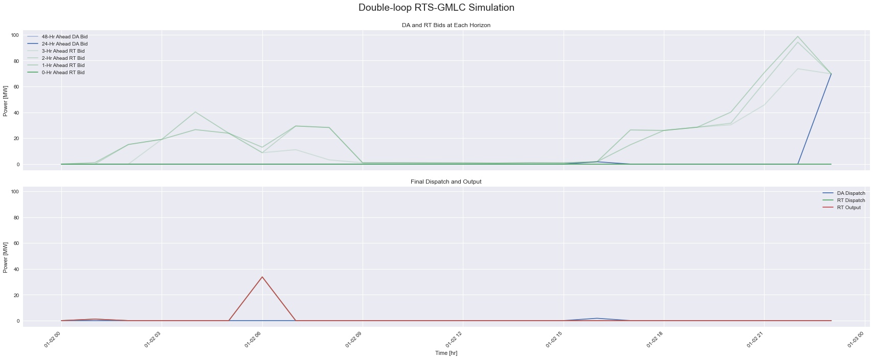
In contrast to the wind plant above which bids its DA resource forecast and its RT resource forecast at $0/MWh marginal cost, the Wind + Battery IES is shifting the times and prices to sell energy. The bidding process for both the DA and RT market take place across multiple horizons within the staggered, forward-rolling UC and ED problems. As the Bidder receives more information about its state within each time horizon, it updates its bids. This is shown in the first plot in the top row, where
the final DA and RT Bid are 24-Hr Ahead DA Bid and 0-Hr Ahead RT Bid. The second row shows the DA Dispatch and RT Dispatch from Prescient, and the delivered RT Output.
[12]:
fig, ax = plt.subplots(2, 1, figsize=(24, 10), sharex=True)
ax[0].plot(time_index, np.append([0] * 24, da_bidder_df[da_bidder_df['Horizon [hr]'] < 24][da_bid_powers].sum(axis=1))[time_slice], color='b', alpha=0.4, label="48-Hr Ahead DA Bid")
ax[0].plot(time_index, da_bidder_df[da_bidder_df['Horizon [hr]'] < 24][da_bid_powers].sum(axis=1)[time_slice], color='b', alpha=1, label="24-Hr Ahead DA Bid")
ax[0].plot(time_index, np.append([0] * 3, rt_bidder_df[rt_bidder_df['Horizon [hr]'] == 3][rt_bid_powers].sum(axis=1))[time_slice], color='g', alpha=0.2, label="3-Hr Ahead RT Bid")
ax[0].plot(time_index, np.append([0] * 2, rt_bidder_df[rt_bidder_df['Horizon [hr]'] == 2][rt_bid_powers].sum(axis=1))[time_slice], color='g', alpha=0.3, label="2-Hr Ahead RT Bid")
ax[0].plot(time_index, np.append([0] * 1, rt_bidder_df[rt_bidder_df['Horizon [hr]'] == 1][rt_bid_powers].sum(axis=1))[time_slice], color='g', alpha=0.4, label="1-Hr Ahead RT Bid")
ax[0].plot(time_index, rt_bidder_df[rt_bidder_df['Horizon [hr]'] == 0]['RT Power 0 [MW]'].values[time_slice], color='g', alpha=1, label="0-Hr Ahead RT Bid")

ax[1].plot(time_index, prescient_df['Dispatch DA'].values[time_slice], color='b', label='DA Dispatch')
ax[1].plot(time_index, prescient_df['Dispatch'].values[time_slice], color='g', label='RT Dispatch')
ax[1].plot(time_index, tracker_df[tracker_df['Horizon [hr]'] == 0][['Power Output [MW]']], color='r', label='RT Output')
ax[1].set_ylim(ax[0].get_ylim())
format_plt(fig, ax, mod_ticks=False, titles=["DA and RT Bids at Each Horizon", "Final Dispatch and Output"], suptitle="Double-loop RTS-GMLC Simulation")
Analyzing the Wind + Battery IES Performance: Tracker and Settlement
The first plot shows the double-loop simulation results. Max power has increased due to battery capacity. In comparison to the original result plotted above, there’s different DA Dispatch due to using RT forecast instead of DA forecast. Also, where there were a few times where the wind plant had negative revenue due to Penalized DA Underdelivered when the RT price was higher than the DA price, here, there is only one instance of being penalized for missing a DA promise. However, there
appears to be more curtailed energy, and the battery is full at least once a day, often more.
The second plot shows the impact on the Generator’s Unit Market Revenue.
[13]:
tracker_df.loc[:, 'Penalized DA Underdelivered'] = 0
prescient_df["Penalized DA Underdelivered"] = ((prescient_df['Dispatch DA'] - prescient_df['Dispatch']) * (prescient_df['LMP'] > prescient_df['LMP DA'])).clip(lower=0).values
tracker_df.loc[tracker_df['Horizon [hr]'] == 0, 'Penalized DA Underdelivered [MW]'] = prescient_df["Penalized DA Underdelivered"].values

fig, ax = plt.subplots(2, 1, figsize=(24, 10), sharex=True)
cols = ["Wind Power Output [MW]", "Battery Power Output [MW]", 'Penalized DA Underdelivered [MW]', "Wind Power to Battery [MW]"]
ax[0].plot(prescient_df['Dispatch DA'].values, drawstyle="steps-mid", label='DA Dispatch [MW]', color='grey')
ax[0].plot(tracker_df.loc[tracker_df['Horizon [hr]'] == 0]['Total Power Output [MW]'].values, drawstyle="steps-mid", label='RT Dispatch [MW]', color='k')
tracker_df.loc[tracker_df['Horizon [hr]'] == 0][cols].plot(kind='bar', width=1, stacked=True, ax=ax[0], color=['b', 'g', 'r', 'c'])

tracker_df.loc[tracker_df['Horizon [hr]'] == 0]['Wind Curtailment [MW]'].plot(kind='bar', width=1, stacked=True, ax=ax[1])
tracker_df.loc[tracker_df['Horizon [hr]'] == 0]["Wind Power to Battery [MW]"].plot(kind='bar', width=1, stacked=True, ax=ax[1], color='c')
ax[1].plot([battery_pmax] * len(time_index), linestyle="dashed", label='Max Stored Power [MWh]', alpha=0.8, color='orange')
ax[1].plot(tracker_df.loc[tracker_df['Horizon [hr]'] == 0]['State of Charge [MWh]'].values / 4, drawstyle="steps-mid", label='Stored Power [MW]', color='y')
format_plt(fig, ax, titles=["Wind + Battery Dispatch and Output", "Wind Curtailment and Battery State-of-Charge"], suptitle="Double-loop RTS-GMLC Simulation")
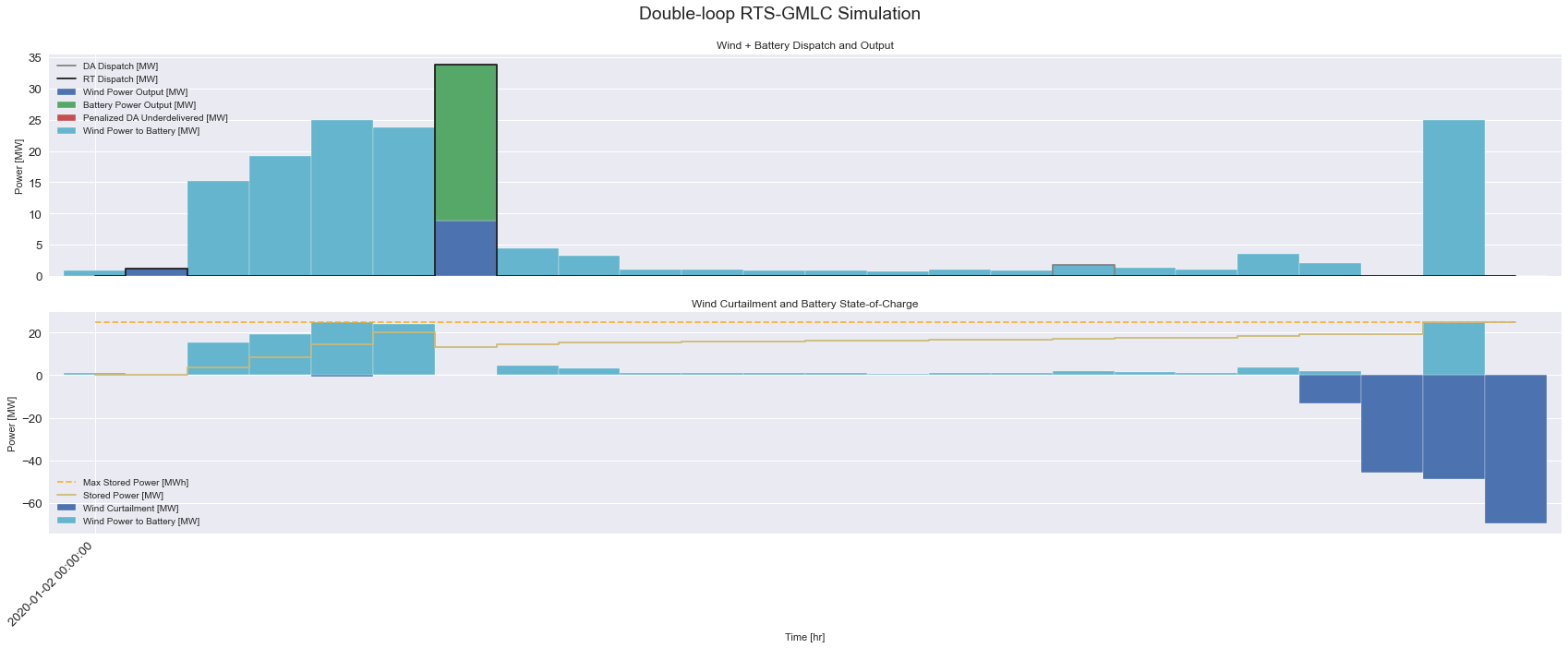
[14]:
fig, ax = plt.subplots(2, 1, figsize=(24, 10), sharex=True)
prescient_df["Penalized DA Underdelivered"].plot(ax=ax[0], color='r', kind='bar', width=1)
ax0 = ax[0].twinx()
ax0.set_yscale('symlog')
ax0.plot(prescient_df['LMP DA'].values, label="LMP DA [$/MWh]")
ax0.plot(prescient_df['LMP'].values, label='LMP RT [$/MWh]')
ax0.legend(loc='upper right')
ax0.set_ylabel("LMP [$/MWh]")
ax0.grid(None)
ax[1].set_yscale('symlog')
ax[1].plot(prescient_df['Unit Market Revenue'].values, color='k', linestyle=':', label="Market Revenue [$]")
ax[1].plot(prescient_df['Unit Market Revenue'].cumsum().values, color='k', label="Cumulative Market Revenue [$]")
format_plt(fig, ax, y_labels=['Power [MW]', 'Revenue [$]'], titles=["LMPs at Missed DA Promises", "Market Revenue"], suptitle="Double-loop RTS-GMLC Simulation")
ax[0].legend(loc='upper left')
[14]:
<matplotlib.legend.Legend at 0x7fd478e5b820>
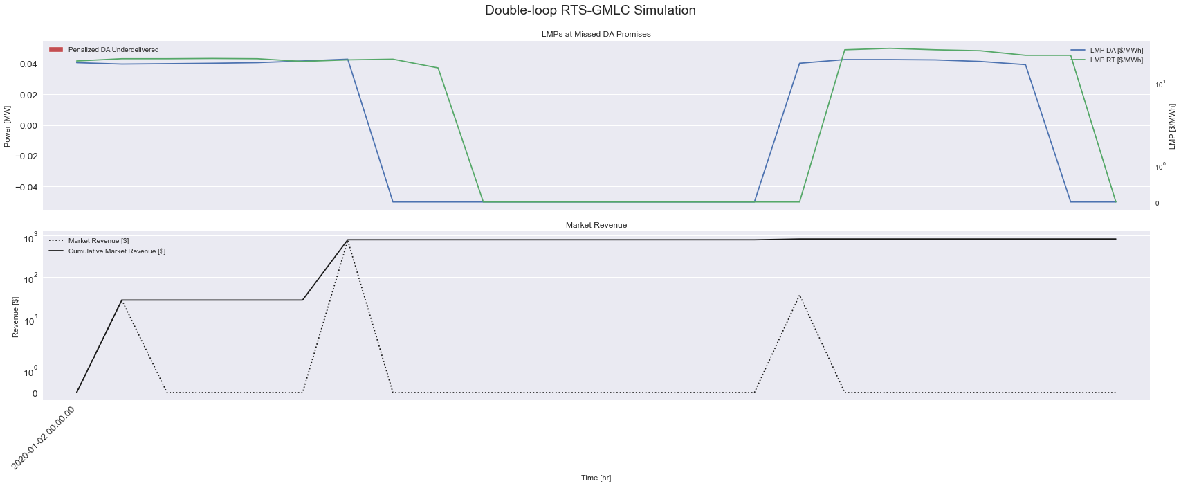
Analyzing the Wind + Battery IES Performance: Comparison to Original RTS-GMLC Simulation
The plots below show the changes in the electricity market which impact the plant’s economic performance and the grid’s production and reliability.
[15]:
fig, ax = plt.subplots(3, 1, figsize=(24, 10), sharex=True)
ax[0].set_yscale('symlog')
ax[0].plot(orig_outputs_df['Unit Market Revenue'].values, color='grey', linestyle=':', label="Orig Market Revenue [$]")
ax[0].plot(orig_outputs_df['Unit Market Revenue'].cumsum().values, color='grey', label="Orig Cumulative Market Revenue [$]")
ax[0].plot(prescient_df['Unit Market Revenue'].values, color='b', linestyle=':', label="Double-loop Market Revenue [$]")
ax[0].plot(prescient_df['Unit Market Revenue'].cumsum().values, color='b', label="Double-loop Cumulative Market Revenue [$]")

ax[1].set_yscale('symlog')
da_rev = orig_outputs_df['Output DA'] * orig_outputs_df['LMP DA']
ax[1].plot(da_rev.values, color='grey', linestyle=':', label="Orig DA Revenue [$]")
ax[1].plot(da_rev.cumsum().values, color='grey', label="Orig Cumulative DA Revenue [$]")
da_rev = prescient_df['Dispatch DA'] * prescient_df['LMP DA']
ax[1].plot(da_rev.values, color='b', linestyle=':', label="Double-loop DA Revenue [$]")
ax[1].plot(da_rev.cumsum().values, color='b', label="Double-loop Cumulative DA Revenue [$]")

ax[2].set_yscale('symlog')
rt_rev = (orig_outputs_df['Output'] - orig_outputs_df['Output DA']) * orig_outputs_df['LMP']
ax[2].plot(rt_rev.values, color='grey', linestyle=':', label="Orig RT Revenue [$]")
ax[2].plot(rt_rev.cumsum().values, color='grey', label="Orig Cumulative RT Revenue [$]")
rt_rev = (tracker_df[tracker_df['Horizon [hr]'] == 0]['Power Output [MW]'] - prescient_df['Dispatch DA']) * prescient_df['LMP']
ax[2].plot(rt_rev.values, color='b', linestyle=':', label="Double-loop RT Revenue [$]")
ax[2].plot(rt_rev.cumsum().values, color='b', label="Double-loop Cumulative RT Revenue [$]")

format_plt(fig, ax, y_labels=['Revenue [$]', "LMP [$/MWh]", "LMP [$/MWh]"], titles=["Total Revenue", 'DA Revenue', 'RT Revenue'], suptitle="Double-Loop vs Original RTS-GMLC Revenue Comparison")
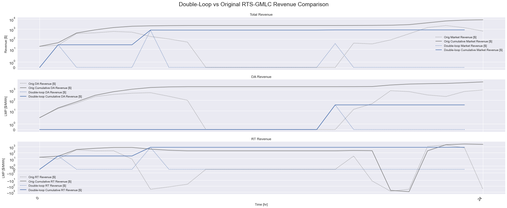
[16]:
fig, ax = plt.subplots(5, 1, figsize=(24, 15), sharex=True)
ax[0].set_yscale('symlog')
ax[0].plot(orig_outputs_df['TotalCosts'].values, color='grey', linestyle=':', label="Orig Production Cost [$]")
ax[0].plot(orig_outputs_df['TotalCosts'].cumsum().values, color='grey', label="Orig Cumulative Production Cost [$]")
ax[0].plot(prescient_df['TotalCosts'].values, color='b', linestyle=':', label="Double-loop Production Cost [$]")
ax[0].plot(prescient_df['TotalCosts'].cumsum().values, color='b', label="Double-loop Cumulative Production Cost [$]")

ax[1].set_yscale('symlog')
ax[1].plot(orig_outputs_df['LoadShedding'].values * -1, color='grey', linestyle=':', label="Orig LoadShedding [MW]")
ax[1].plot(orig_outputs_df['LoadShedding'].cumsum().values * -1, color='grey', label="Orig Cumulative LoadShedding [MW]")
ax[1].plot(prescient_df['LoadShedding'].values * -1, color='b', linestyle=':', label="Double-loop LoadShedding [MW]")
ax[1].plot(prescient_df['LoadShedding'].cumsum().values * -1, color='b', label="Double-loop Cumulative LoadShedding [MW]")

ax[2].set_yscale('symlog')
ax[2].plot(orig_outputs_df['Curtailment'].values, color='grey', linestyle=':', label="Orig Curtailment [MW]")
ax[2].plot(orig_outputs_df['Curtailment'].cumsum().values, color='grey', label="Cumulative Orig Curtailment [MW]")
ax[2].plot(tracker_df[tracker_df['Horizon [hr]'] == 0]['Wind Curtailment [MW]'].values, color='b', linestyle=':', label="Double-loop Curtailment [MW]")
ax[2].plot(tracker_df[tracker_df['Horizon [hr]'] == 0]['Wind Curtailment [MW]'].cumsum().values, color='b', label="Double-loop Cumulative Curtailment [MW]")

ax[3].set_yscale('symlog')
ax[3].plot(orig_outputs_df['LMP DA'].values, color='grey', label="Orig DA LMPs [$]")
ax[3].plot(prescient_df['LMP DA'].values, color='b', label="Double-loop DA LMPs [$]")

ax[4].set_yscale('symlog')
ax[4].plot(orig_outputs_df['LMP'].values, color='grey', label="Orig RT LMPs [$]")
ax[4].plot(prescient_df['LMP'].values, color='b', label="Double-loop RT LMPs [$]")

format_plt(fig, ax, y_labels=['Cost [$]', "Power [MW]", "Power [MW]", "LMP [$/MWh]", "LMP [$/MWh]"], titles=["Total Production Cost", 'Load Shed', 'Curtailment', 'DA LMPs', 'RT LMPs'], suptitle="Double-Loop vs Original RTS-GMLC Grid Comparison")